Reaching Dataset Example
A demonstration of Spykes’ functionality using the reaching dataset.
import numpy as np
import pandas as pd
from spykes.plot.neurovis import NeuroVis
from spykes.ml.neuropop import NeuroPop
from spykes.io.datasets import load_reaching_data
from spykes.utils import train_test_split
import matplotlib.pyplot as plt
Initialization
Download Reaching Dataset
Load Data
reach_data = load_reaching_data()

print('dataset keys:', reach_data.keys())
print('events:', reach_data['events'].keys())
print('features', reach_data['features'].keys())
print('number of PMd neurons:', len(reach_data['neurons_PMd']))
print('number of M1 neurons:', len(reach_data['neurons_M1']))
Out:
('dataset keys:', ['neurons_M1', 'neurons_PMd', 'events', 'features'])
('events:', ['rewardTime', 'goCueTime', 'targetOnTime'])
('features', ['endpointOfReach', 'reward'])
('number of PMd neurons:', 195)
('number of M1 neurons:', 219)
Part I: NeuroVis
Instantiate Example PMd Neuron
neuron_number = 91
spike_times = reach_data['neurons_PMd'][neuron_number - 1]
neuron_PMd = NeuroVis(spike_times, name='PMd %d' % neuron_number)
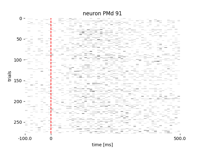
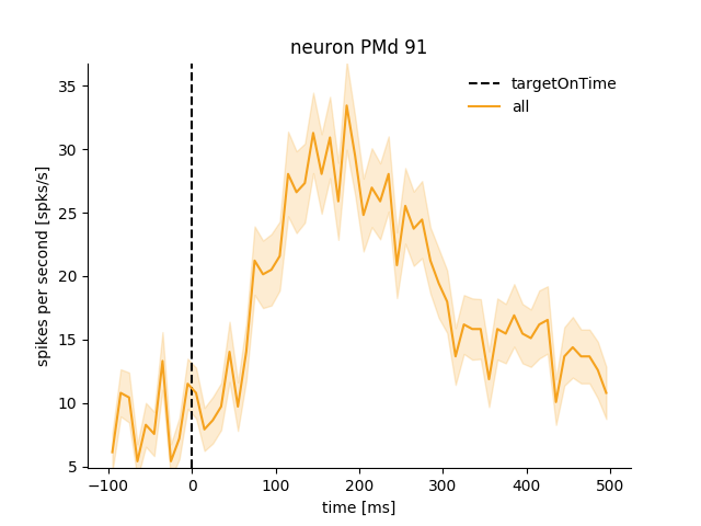
Raster plot and PSTH aligned to target onset
neuron_PMd.get_raster(event='targetOnTime', df=reach_data['events'])
neuron_PMd.get_psth(event='targetOnTime', df=reach_data['events'])
Let’s put the data into a DataFrame
Events
data_df = pd.DataFrame()
events = ['targetOnTime', 'goCueTime', 'rewardTime']

for i in events:
    data_df[i] = np.squeeze(reach_data['events'][i])


data_df[events].head()
Features
data_df['endpointOfReach'] = np.squeeze(
    reach_data['features']['endpointOfReach'])
data_df['reward_code'] = reach_data['features']['reward']

features = ['endpointOfReach', 'reward_code']
data_df[features].head()
Let’s visualize PSTHs separated by conditions
Example 1: Reward vs No Reward
# We could use 'reward_code' but let's create a boolean feature for reward
data_df['reward'] = data_df['reward_code'].map(
    lambda s: {32: True, 34: False, '': np.nan}[s])
data_df.head()
Plot PSTH
psth = neuron_PMd.get_psth(event='rewardTime',
                           conditions='reward',
                           df=data_df)
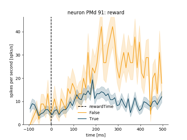
Make it look nicer
plt.figure(figsize=(10, 5))
psth = neuron_PMd.get_psth(event='rewardTime',
                           conditions='reward',
                           df=data_df,
                           window=[-200, 600],
                           binsize=20,
                           event_name='Reward Time')

plt.title('neuron %s: Reward' % neuron_PMd.name)
plt.show()
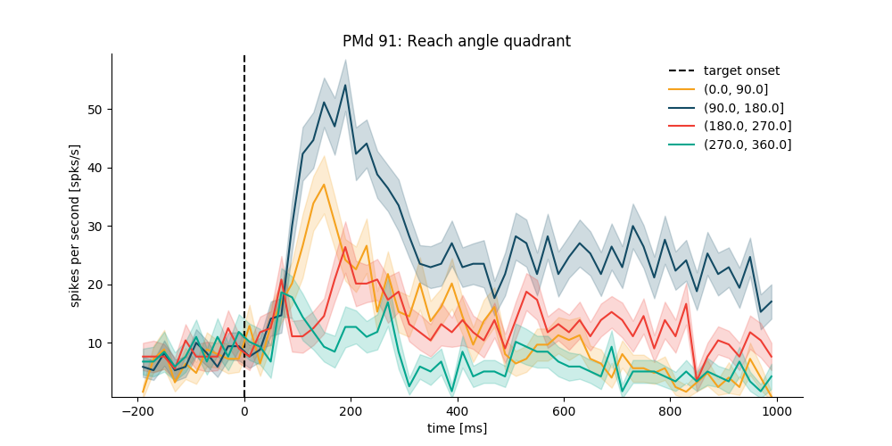
Example 2: according to quadrant of reaching direction
data_df['endpointOfReach_quad'] = pd.cut(
    data_df['endpointOfReach'], np.linspace(0, 360, 5))
data_df[['endpointOfReach', 'endpointOfReach_quad']].head()
plt.figure(figsize=(10, 5))
psth_PMd = neuron_PMd.get_psth(event='targetOnTime',
                               conditions='endpointOfReach_quad',
                               df=data_df,
                               window=[-200, 1000],
                               binsize=20,
                               event_name='target onset')

plt.title('%s: Reach angle quadrant' % neuron_PMd.name)
plt.show()
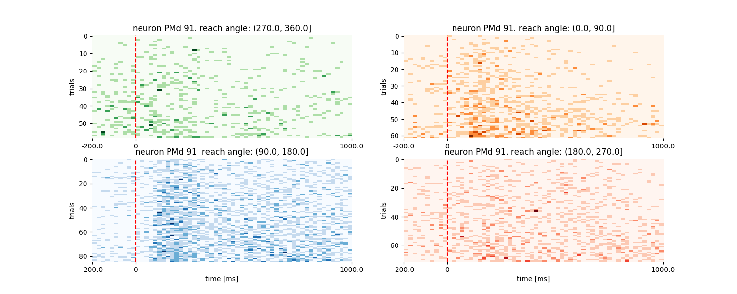
Raster plots for the same neuron and conditions
# get rasters
rasters_PMd = neuron_PMd.get_raster(event='targetOnTime',
                                    conditions='endpointOfReach_quad',
                                    df=data_df,
                                    window=[-200, 1000],
                                    binsize=20,
                                    plot=False)


# plot rasters
plt.figure(figsize=(15, 6))
plot_order = np.array([2, 3, 4, 1])
cmap = ['Oranges', 'Blues', 'Reds', 'Greens']
for i, cond_id in enumerate(np.sort(rasters_PMd['data'].keys())):
    plt.subplot(2, 2, plot_order[i])
    neuron_PMd.plot_raster(rasters_PMd,
                           cond_id=cond_id,
                           cmap=cmap[i],
                           cond_name='reach angle: %s' % cond_id,
                           sortby='rate', sortorder='ascend')
    if plot_order[i] < 3:
        plt.xlabel('')
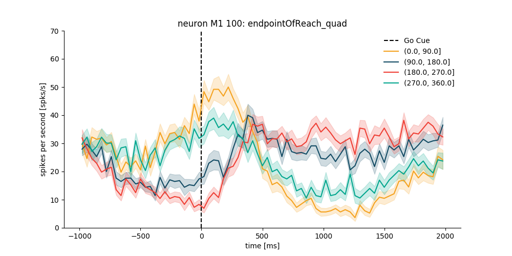
Example 3: Same as Example 2 but for an M1 neuron and aligned at goCueTime
neuron_number = 100
spike_times = reach_data['neurons_M1'][neuron_number - 1]
neuron_M1 = NeuroVis(spike_times, name='M1 %d' % neuron_number)
plt.figure(figsize=(10, 5))
psth_M1 = neuron_M1.get_psth(event='goCueTime',
                             df=data_df,
                             conditions='endpointOfReach_quad',
                             window=[-1000, 2000],
                             binsize=40,
                             plot=True,
                             ylim=[0, 70],
                             event_name='Go Cue')
plt.show()
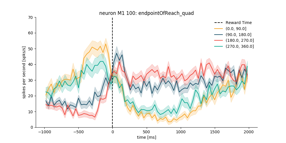
Example 4: sorted by direction only for the trials with reward
# use standard pandas filtering to isolate trials of interest
trials_df = data_df[data_df['reward'] == True]
trials_df.head()
plt.figure(figsize=(10, 5))
psth_M1 = neuron_M1.get_psth(event='rewardTime',
                             conditions='endpointOfReach_quad',
                             df=trials_df,
                             window=[-1000, 2000],
                             binsize=40,
                             ylim=[0, 70],
                             event_name='Reward Time'
                             )
plt.show()
One last thing before moving on to spykes.neuropop We can use get_spikecounts() to count the number of spikes within a certain time window relative to event onset
spike_counts = neuron_PMd.get_spikecounts(
    'targetOnTime', df=data_df, window=[0, 1200])
conditions_names = np.unique(data_df['endpointOfReach_quad'])
conditions_names = conditions_names[[0, 3, 1, 2]]
conditions_names
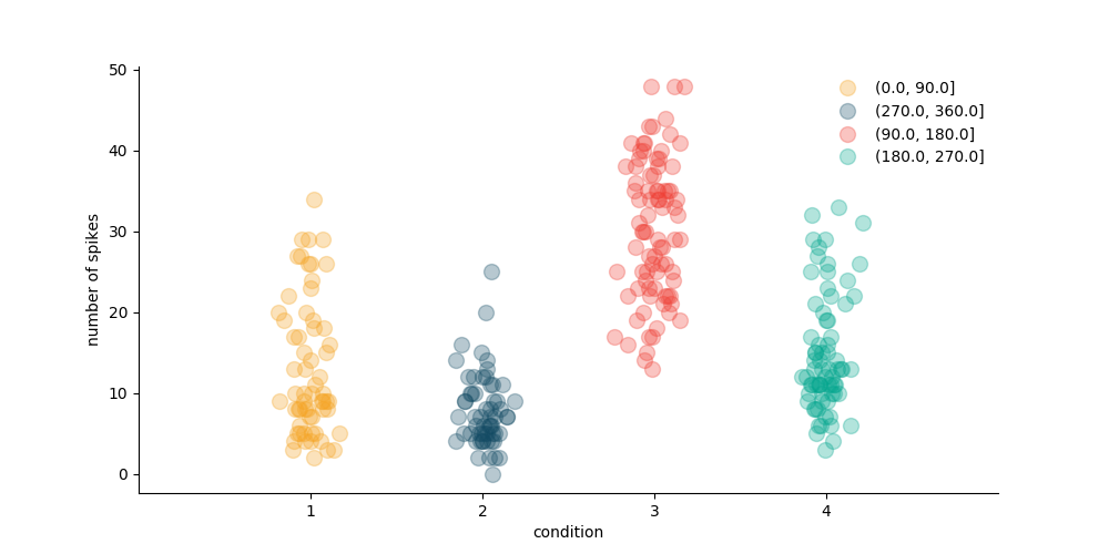
Let’s visualize the spike counts per trial for each condition
colors = ['#F5A21E', '#134B64', '#EF3E34', '#02A68E']

plt.figure(figsize=(10, 5))
for i, cond in enumerate(conditions_names):
    idx = np.where(data_df['endpointOfReach_quad'] == cond)[0]
    x_noise = 0.08 * np.random.randn(np.size(idx))
    plt.plot(i + x_noise + 1, spike_counts[idx], '.', color=colors[i],
             alpha=0.3, markersize=20)

plt.xlabel('condition')
plt.ylabel('number of spikes')
plt.xlim([0, 5])
plt.xticks(np.arange(np.size(conditions_names)) + 1)
ax = plt.gca()
ax.spines['top'].set_visible(False)
ax.spines['right'].set_visible(False)
plt.tick_params(axis='y', right='off')
plt.tick_params(axis='x', top='off')
plt.legend(conditions_names, frameon=False)
plt.show()
Part II: NeuroPop
Organize data as preferred features and spike counts (x Y)
Extract reach direction x
# Get reach direction, ensure it is between [-pi, pi]
x = np.arctan2(np.sin(reach_data['features']['endpointOfReach'] *
               np.pi / 180.0),
               np.cos(reach_data['features']['endpointOfReach'] *
               np.pi / 180.0))
Extract M1 spike counts Y
- Select only neurons above a threshold firing rate
- Align spike counts to the GO cue
- Use the convenience function
`get_spikecounts()`from`NeuroVis`
# Select only high firing rate neurons
M1_select = list()
threshold = 10.0

# Specify timestamps of events to which trials are aligned
align = 'goCueTime'

# Specify a window of around the go cue for spike counts
window = [0., 500.]  # milliseconds

# Get spike counts
Y = np.zeros([x.shape[0], len(reach_data['neurons_M1'])])

for n in range(len(reach_data['neurons_M1'])):
    this_neuron = NeuroVis(spiketimes=reach_data['neurons_M1'][n])
    Y[:, n] = np.squeeze(
        this_neuron.get_spikecounts(event=align, df=data_df, window=window))

    # Short list a few high-firing neurons
    if this_neuron.firingrate > threshold:
        M1_select.append(n)

# Rescale spike counts to units of spikes/s
Y = Y / float(window[1] - window[0]) * 1e3

# How many neurons shortlisted?
print('%d M1 neurons had firing rates over %4.1f spks/s' %
      (len(M1_select), threshold))
Out:
107 M1 neurons had firing rates over 10.0 spks/s
Split into train and test sets
np.random.seed(42)
(Y_train, Y_test), (x_train, x_test) = train_test_split(Y, x, percent=0.33)
Create an instance of NeuroPop
pop = NeuroPop(n_neurons=len(M1_select),
               tunemodel='gvm',
               n_repeats=3,
               verbose=False)

# Let's fit tuning curves to the population
# ~~~~~~~~~~~~~

pop.fit(np.squeeze(x_train), Y_train[:, M1_select])
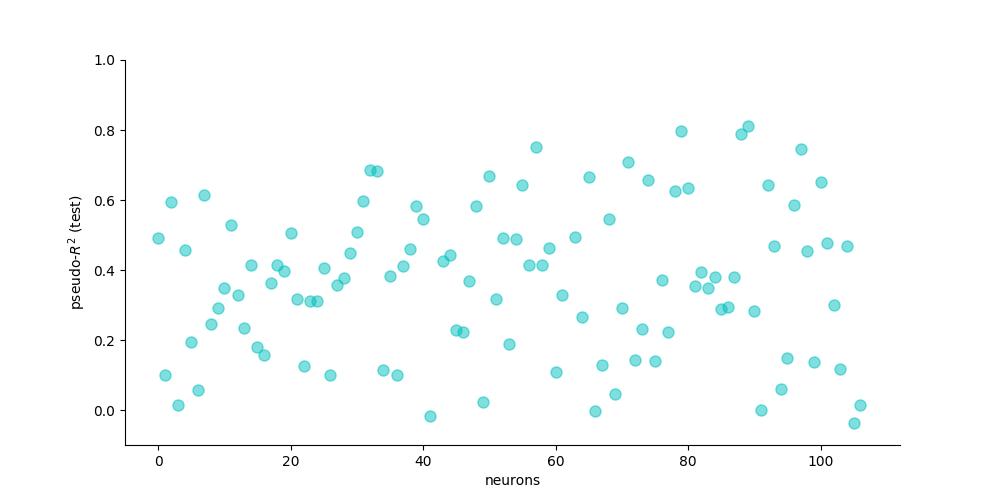
Predict firing rates
Yhat_test = pop.predict(np.squeeze(x_test))
Score the prediction
# calculate and plot the pseudo R2
Ynull = np.mean(Y_train[:, M1_select], axis=0)
pseudo_R2 = pop.score(
    Y_test[:, M1_select], Yhat_test, Ynull, method='pseudo_R2')

plt.figure(figsize=(10, 5))
plt.plot(pseudo_R2, 'co', markeredgecolor='c', alpha=0.5, markersize=8)
plt.xlim([-5, len(M1_select) + 5])
plt.ylim([-0.1, 1])
plt.xlabel('neurons')
plt.ylabel('pseudo-$R^2$ (test)')
ax = plt.gca()
ax.spines['top'].set_visible(False)
ax.spines['right'].set_visible(False)
plt.tick_params(axis='y', right='off')
plt.tick_params(axis='x', top='off')
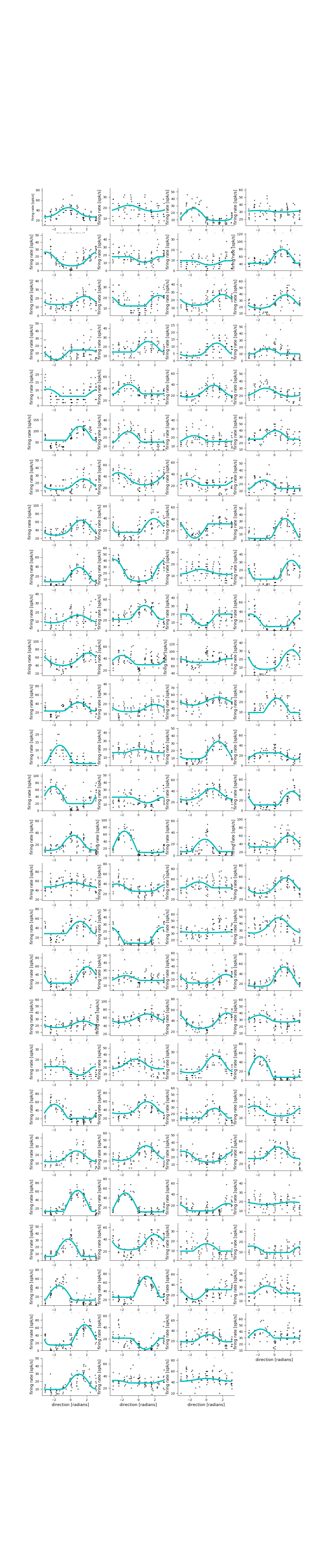
Visualize tuning curves
plt.figure(figsize=[15, 70])

for neuron in range(len(M1_select)):
    plt.subplot(27, 4, neuron + 1)
    pop.display(x_test, Y_test[:, M1_select[neuron]], neuron=neuron,
                ylim=[0.8 * np.min(Y_test[:, M1_select[neuron]]),
                1.2 * np.max(Y_test[:, M1_select[neuron]])])
    # plt.axis('off')

plt.show()
Decode reach direction from population vector
xhat_test = pop.decode(Y_test[:, M1_select])
Visualize decoded reach direction
plt.figure(figsize=[6, 5])

plt.plot(x_test, xhat_test, 'k.', alpha=0.5)
plt.xlim([-1.2 * np.pi, 1.2 * np.pi])
plt.ylim([-1.2 * np.pi, 1.2 * np.pi])
plt.xlabel('Ground truth [radians]')
plt.ylabel('Decoded [radians]')
plt.tick_params(axis='y', right='off')
plt.tick_params(axis='x', top='off')
ax = plt.gca()
ax.spines['top'].set_visible(False)
ax.spines['right'].set_visible(False)

plt.figure(figsize=[15, 5])
jitter = 0.2 * np.random.rand(x_test.shape[0])
plt.subplot(121, polar=True)
plt.plot(x_test, np.ones(x_test.shape[0]) + jitter, 'ko', alpha=0.5)
plt.title('Ground truth')

plt.subplot(122, polar=True)
plt.plot(xhat_test, np.ones(xhat_test.shape[0]) + jitter, 'co', alpha=0.5)
plt.title('Decoded')
plt.show()
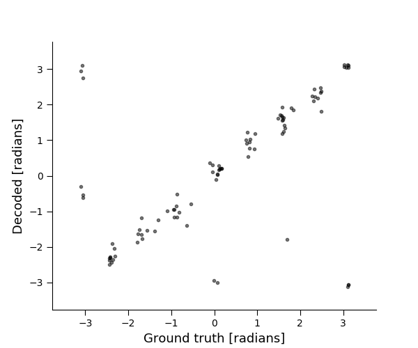
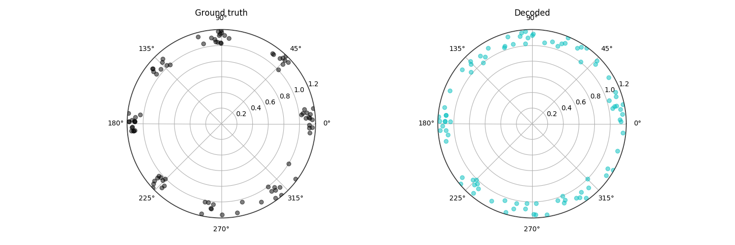
Score decoding performance
circ_corr = pop.score(x_test, xhat_test, method='circ_corr')
print('Circular Correlation: %f' % (circ_corr))
cosine_dist = pop.score(x_test, xhat_test, method='cosine_dist')
print('Cosine Distance: %f' % (cosine_dist))
Out:
Circular Correlation: 0.785828
Cosine Distance: 0.851796
Total running time of the script: ( 1 minutes 24.141 seconds)