Neuropop Example

A demonstration of Neuropop using simulated data

import numpy as np
import matplotlib.pyplot as plt

from spykes.ml.neuropop import NeuroPop
from spykes.utils import train_test_split

Create a NeuroPop object

n_neurons = 10
pop = NeuroPop(n_neurons=n_neurons, tunemodel='glm')

Simulate a population of neurons

n_samples = 1000
x, Y, mu, k0, k, g, b = pop.simulate(pop.tunemodel, n_samples=n_samples,
                                     winsize=400.0)

Split into training and testing sets

np.random.seed(42)
(Y_train, Y_test), (x_train, x_test) = train_test_split(Y, x, percent=0.5)

Fit the tuning curves with gradient descent

pop.fit(x_train, Y_train)

Predict the population activity with the fit tuning curves

Yhat_test = pop.predict(x_test)

Score the prediction

Ynull = np.mean(Y_train, axis=0)
pseudo_R2 = pop.score(Y_test, Yhat_test, Ynull, method='pseudo_R2')
print(pseudo_R2)

Out:

[0.012898436115752809, 0.87906982333904071, 0.64953551355040173, 0.71023596752501739, 0.8625152869878786, 0.19022506746859158, 0.87195203613890515, 0.52223737867131592, 0.87889200248158028, 0.89802770436521395]

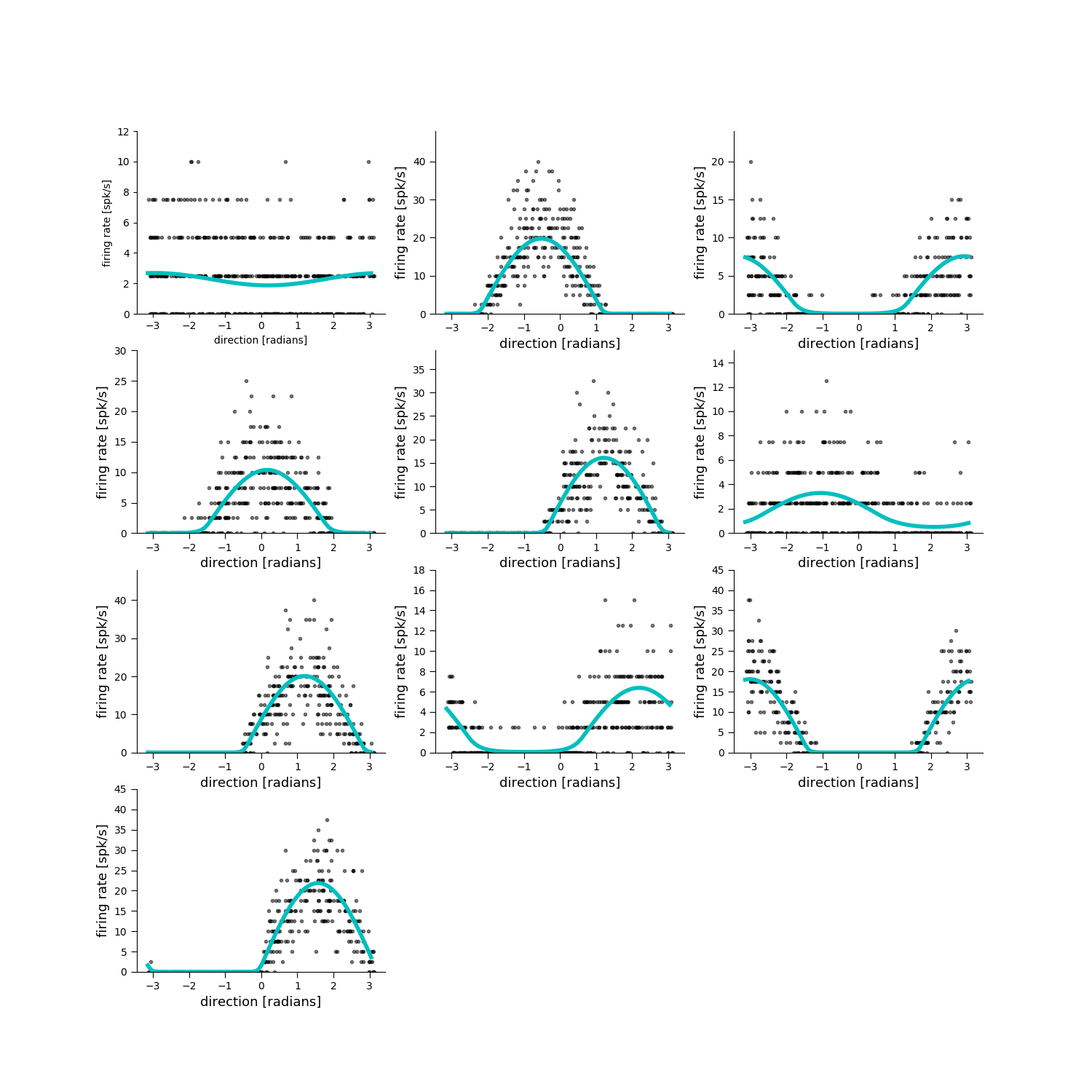
Plot the simulated and fit tuning curves

plt.figure(figsize=[15, 15])

for neuron in range(pop.n_neurons):
    plt.subplot(4, 3, neuron + 1)
    pop.display(x_test, Y_test[:, neuron], neuron=neuron,
                ylim=[0.8 * np.min(Y_test[:, neuron]), 1.2 *
                np.max(Y_test[:, neuron])])

plt.show()

Decode feature from the population activity

xhat_test = pop.decode(Y_test)

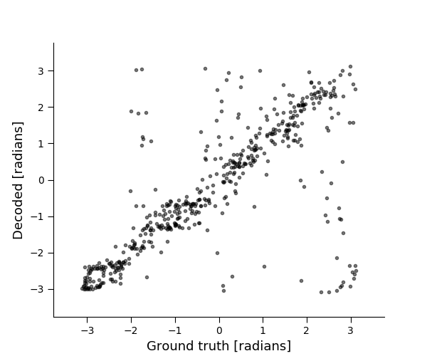
Visualize ground truth vs. decoded estimates

plt.figure(figsize=[6, 5])

plt.plot(x_test, xhat_test, 'k.', alpha=0.5)
plt.xlim([-1.2 * np.pi, 1.2 * np.pi])
plt.ylim([-1.2 * np.pi, 1.2 * np.pi])
plt.xlabel('Ground truth [radians]')
plt.ylabel('Decoded [radians]')
plt.tick_params(axis='y', right='off')
plt.tick_params(axis='x', top='off')
ax = plt.gca()
ax.spines['top'].set_visible(False)
ax.spines['right'].set_visible(False)

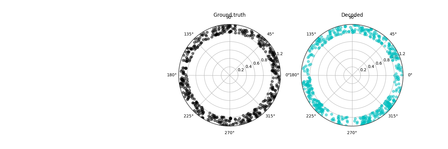
plt.figure(figsize=[15, 5])
jitter = 0.2 * np.random.rand(x_test.shape[0])
plt.subplot(132, polar=True)
plt.plot(x_test, np.ones(x_test.shape[0]) + jitter, 'ko', alpha=0.5)
plt.title('Ground truth')

plt.subplot(133, polar=True)
plt.plot(xhat_test, np.ones(xhat_test.shape[0]) + jitter, 'co', alpha=0.5)
plt.title('Decoded')
plt.show()

• 
• 

Score decoding performance

# Circular correlation
circ_corr = pop.score(x_test, xhat_test, method='circ_corr')
print('Circular correlation: %f' % (circ_corr))

Out:

Circular correlation: 0.743451

# Cosine distance
cosine_dist = pop.score(x_test, xhat_test, method='cosine_dist')
print('Cosine distance: %f' % (cosine_dist))

Out:

Cosine distance: 0.797382

Total running time of the script: ( 0 minutes 22.722 seconds)